.ipynb .pdf

repository open issue suggest edit

Binder Live Code

On this page

Steady Level Flight

The discipline of Aircraft Flight Mechanics requires the formulation of relationships between aircraft forces, and aircraft motion. In order to define motion, it was necessary to define the different airspeeds in the preceding section.

Aircraft have six degrees of freedom - three translational (\(x, y, z\)), and three rotational (\(\phi, \theta, \psi\)), and in order to develop the expressions describing aircraft flight, nine coupled equations are required. This course will get to that point, and those equations will derived and utilised - but before that, some really handy relationships can be defined for flight constrained to a single direction.

The simplest flight regime is best to start with, which is steady, level (meaning no change in altitude) flight.

A word about SLUF…

Sometimes you may see this flight regime caled SLUF, standing for Steady Level Unaccellerated Flight. I don’t particularly like this acronym as:

• Steady means unaccelerated, so it’s tautologous

• There’s another, arguably better definition for SLUF

Let’s explore what this regime means, and the assumptions we make

• We assume that the aircraft is a point mass, whereby we assume that the aircraft dimensions are negligible when compared to the dimensions of motion.

• Steady flight means no acceleration, so we can infer from Newton’s first law that the sum of forces acting on the aircraft is zero \(\sum\vec{F}=0\) . This is the equilibrium steady flight condition.

The definition of forces on the aircraft can change depending on the purpose - and it is only be convention that we define lift and drag in the directions we do.

The semantics notwithstanding, it is traditional to define four mutually-orthogonal forces - see Equilibrium Forces.

• Two aerodynamic; lift and drag.

• One propulsive; thrust.

• One inertial; weight.

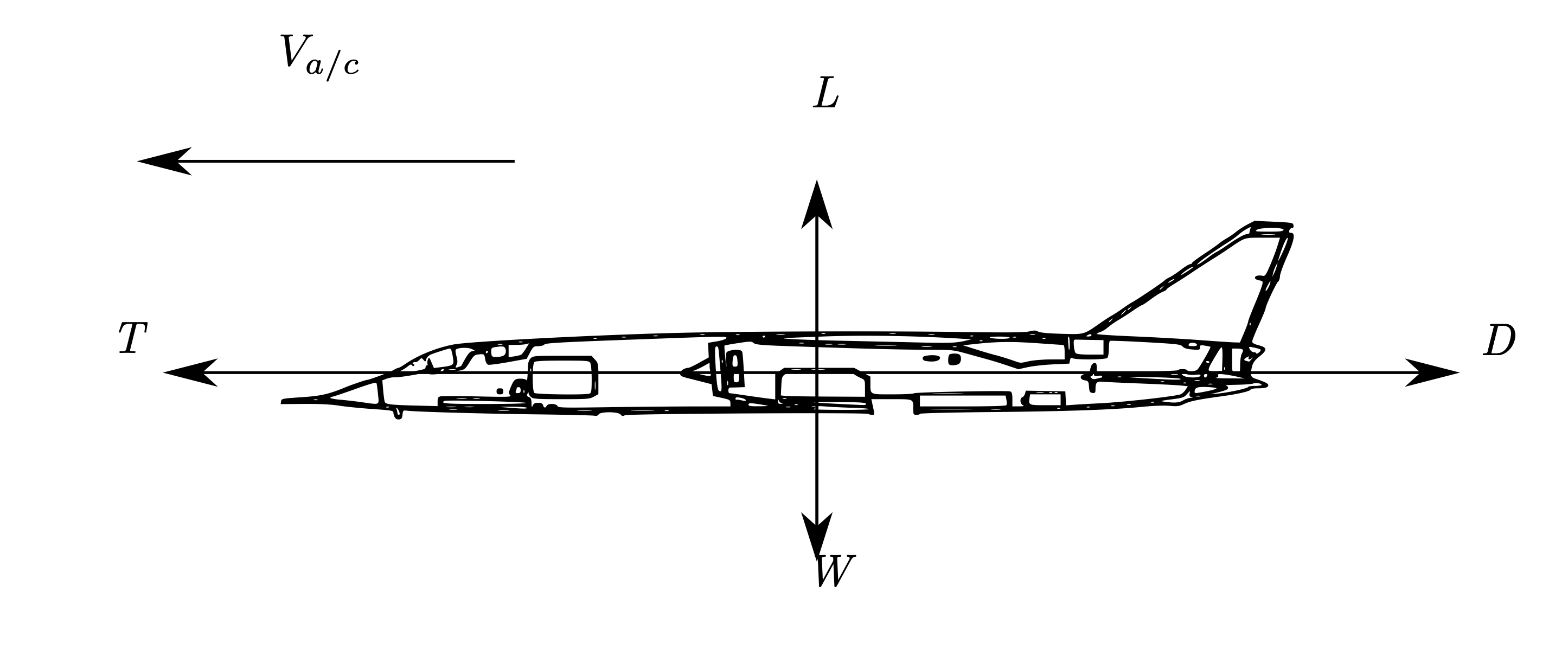
Fig. 18 Equilibrium Forces

For this regime, it is further assumed that the aerodynamic incidence is small, and that the thrust offset is negligible. Therefore we assume that lift and weight are perpendicular to aircraft motion, and that thrust and drag are parallel to aircraft motion.

Vertical Forces

Looking at the vertical forces, \(\sum F_z =0\), therefore \(L=W\):

\[C_L = \frac{L}{\tfrac{1}{2}\rho V^2S}\]

\[ = \frac{W}{\tfrac{1}{2}\rho V^2S}\]

rearranging to find flight speed:

(5)\[V = \sqrt{\frac{\frac{W}{S}}{\tfrac{1}{2}\rho C_L}}\]

Equation (5) is the Aircraft Speed Equation for steady level flight, and some basic aerodynamic behaviour may be inferred from it:

• Slower flight is possible by reducing wing loading - reducing aircraft mass, or increasing wing area. Or by increasing \(C_L\) - increasing \(\alpha\)

• The minimum possible flight speed occurs at \(C_{L_{max}}\) - just before stall

• Flight speed may be increased by reducing \(\rho\) - by flying at increased altitude

Stall speed

From (5), the stall speed may be determined if \(C_{L_{max}}\) is known.

Longitudinal Forces

Looking at the longitudinal forces, \(\sum F_x =0\), therefore \(T=D\):

\[\begin{split}\begin{aligned} C_D &= \frac{D}{\tfrac{1}{2}\rho V^2S}\nonumber\\ &= \frac{T}{\tfrac{1}{2}\rho V^2S}\nonumber\end{aligned}\end{split}\]

Drag estimation is complex, and can be performed via a variety of means from datasheets, CFD, wind tunnel testing or - more commonly - a combination of all. A good breakdown of drag sources is given by MacCormick[Mac95], and a reproduction of the breakdown given is found in the dropdown below - but this is far beyond the complexity required for Aircraft Performance.

Drag Breakdown (well beyond what we need, but included for reference)

The following is an extract from MacCormick[Mac95] [pp. 162-163]:

Induced Drag The drag that results from the generation of a trailing vortex system downstream of a lifting surface of finite aspect ratio.

Parasite Drag The total drag of an airplane minus the induced drag. Thus, it is the drag not directly associated with the production of lift. The parasite drag is composed of many drag components, the definitions of which follow.

Skin Friction Drag The drag on a body resulting from viscous shearing stresses over its wetted surface.

Form Drag (Sometimes Called Pressure Drag) The drag on a body resulting from the integrated effect of the static pressure acting normal to its surface resolved in the drag direction.

Interference Drag The increment in drag resulting from bringing two bodies in proximity to each other. For example, the total drag of a wing-fuselage combination will usually be greater than the sum of the wing drag and fuselage drag independent of each other.

Trim Drag The increment in drag resulting from the aerodynamic forces required to trim the airplane about its center of gravity. Usually this takes the form of added induced and form drag on the horizontal tail.

Profile Drag Usually taken to mean the total of the skin friction drag and form drag for a two-dimensional airfoil section.

Cooling Drag The drag resulting from the momentum lost by the air that passes through the power plant installation for purposes of cooling the engine, oil, and accessories.

Base Drag The specific contribution to the pressure drag attributed to the blunt after-end of a body.

Wave Drag Limited to supersonic flow, this drag is a pressure drag resulting from non-canceling static pressure components to either side of a shock wave acting on the surface of the body from which the wave is emanating.

In flight performance, we assume that the aircraft is operating in the region of linear aerodynamics, and utilise a drag model as given by Equation (6):

(6)\[\begin{split} \underbrace{C_D}_{\text{Total Drag}} = \underbrace{C_{D0}}_{\substack{\text{Zero incidence} \\ \text{drag}}} + \underbrace{K\cdot C_L^2}_{\substack{\text{Induced Drag +} \\ \text{$\alpha$-dependent form drag}}}\end{split}\]

where

\[ K=\frac{k}{\pi AR} = \frac{1}{\pi\,e_0\,AR}\]

The first term represents the drag that is independent of aerodynamic incidence, whilst the second term is proportional to \(C_L^2\), which represents the induced drag and the component of form drag that varies with incidence.

The parameter \(k\sim 1.1-1.4\) for most aircraft, and \(AR\) is the wing aspect ratio \(AR = \frac{b^2}{S}\). \(K\), \(C_{D0}\) usually assumed constant, but can depend on:

• configuration changes (flap deployment)

• Reynolds Number (speed and height)

• Compressibility (shock waves)

Or sometimes can be presented as the Oswold efficiency factor, \(e_0\), which can be related to \(K\) through the aspect ratio.

Equation (6) assumes that the minimum drag occurs at zero lift. This is the case for a symmetric aerofoil, but not for a cambered one. Since most airfcraft have a cambered wing, Equation (6) should be modified to

\[C_D = C_{D, min} + K\left(C_L - C_{L0}\right)^2\]

The second equation is more realistic for real aircraft - but adds complexity to the algebra, and the difference between \(C_{D0}\) and \(C_{D,min}\) is very small even for wings of moderate camber[And99]. For simplicity, Equation (6) will be used in development of the Aircraft Performance Equations.

Equation (5) and Equation (6) underpin the basics of aircraft performance.

Drag Polar

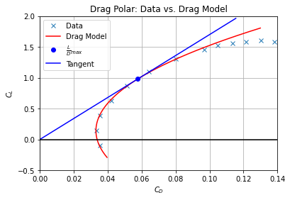
The relationship between lift and drag is given through the aircraft drag polar - often plotted as \(C_L\) vs \(C_D\). Values for \(C_L\) and \(C_D\) are commonplace in the literature - a quick search yielded data for the Cessna 172S [Hab16].

You will see that the drag model works well for low values of lift - that is, in the linear aerodynamic region. The behaviour at the ‘bottom’ of the curve is sometimes called the ‘drag bucket’ - and I spent many years collecting these data in a wind tunnel.

The drag polar shows the aerodynamic efficiency of a given aircraft - that is, it represents the lift-to-drag ratio. You can find the best (highest) lift to drag ratio as the tangent of a line drawn from the origin to the curve.

It would be great to be able to find the best lift to drag ratio without having to draw the drag polar. If you looka the source code for the image below, then it’s obvious that I haven’t drawn the tangent to find the best lift to drag ratio - rather I have drawn the tangent after having found the best lift to drag ratio.

Expand the code to see the source data and coefficients used in the drag model.

# Aircraft Drag polar
import numpy as np
import matplotlib.pyplot as plt

# Data for this graph has been taken from here: 
# https://www.researchgate.net/figure/Figure-A10-Drag-polar-for-the-Cessna-172S-This-plot-is-created-for-NACA-2412-airfoil_fig25_328578766

# Discrete points:
Cd = np.array([0.033099, 0.035185, 0.035214, 0.041961, 0.051143,\
0.064192, 0.080106, 0.096683, 0.104613, 0.11364, 0.121425, 0.130259, 0.138232])
Cl = np.array([0.1454, -0.09219, 0.38303, 0.6238, 0.86305, 1.09772,\
1.31082, 1.45757, 1.51784, 1.55342, 1.58437, 1.60452, 1.58455])

a = np.asarray([Cl, Cd])
np.savetxt("CessnaDragPolar.csv", a.transpose(), delimiter=",", header="Cl, Cd")

plt.plot(Cd, Cl, 'x', label='Data')

# Put the drag model on top
Clvector = np.linspace(min(Cl) - .2, max(Cl) + .2, int(1e3))
Cd0 = 0.033
Cl0 = 0.14
K = 0.035
Cdvector = Cd0 + K*(Clvector - Cl0)**2
plt.plot(Cdvector, Clvector, '-r', label="Drag Model")
plt.legend
plt.xlabel('$C_D$')
plt.ylabel('$C_L$')

plt.title('Drag Polar: Data vs. Drag Model');

# Determine minimum drag
Clmind = np.sqrt(Cd0/K + Cl0**2)
Cdmind =  Cd0 + K*(Clmind - Cl0)**2

# plot it
plt.plot(Cdmind, Clmind, 'ob', label="$\\frac{L}{D}_{max}$")

# show that this is the tangent
plt.plot([0, Cdmind*2], [0, Clmind*2], '-b', label="Tangent")
plt.gca().set_xlim(0, .14);
plt.gca().set_ylim(-.5, 2);
plt.gca().grid('on')
plt.axhline(0, color='black');

# Legend
plt.legend();

Best lift to drag ratio

The highest lift to drag ratio gives the position of best aerodynamic efficiency, and sets the best glide ratio for an aircraft.

In the following, the values of \(C_L\) and \(C_D\) for optimum aerodynamic efficiency - but before diving into the mathematics, some consideration of their significance might be necessary for some readers.

Why do we want to know \(C_L\)?

In the aviation world, pilots tend to be excellent at intuiting flight physics - and being able to relate control movement to aircraft flight, without needed to understand the physics (often in spite of thinking they do).

By contrast, aerospace engineers tend to be be excellent and understanding the mathematics of flight physics - without any consideration of the physical significance of what they are actually deriving. By way of an example ask yourself - ‘what control would you change to effect an altitude change?’, and if your answer is simply ‘pull the stick/yoke back’, then this highlights a misunderstanding of the aircraft controls and physics. In reality, it would be a combination of throttle and stick, but fundamentally you need to gain potential energy which requires an increase in energy from somewhere, i.e., the engine.

---

Back to the problem at hand:

Consider what “to fly at a \(C_L=X\)” actually means - the pilot controls the pitch of the aircraft using fore-aft motion of the stick/yoke. A change in pitch changes the angle of attack of the aircraft, which changes the aircraft lift coefficient.

In reality, a pilot will not tend to consider the numerical value of \(\alpha\) they are flying at - and they are even less likely to know the \(C_L\) of the aircraft under a given flight regime.

For a given \(C_L\), the aircraft speed determines the dimensional value of lift being produced. If \(L=W\), this is steady level flight. If \(L>W\), the aircraft climbs, if \(L<W\), the aircraft descends.

Through a combination of throttle setting, and elevator deflection (stick fore/aft), steady flight can be achieved. Again - the pilot probably isn’t considering the \(C_L\) value, and won’t know whether they’re at the best lift to drag ratio or not.

So - there is a certain speed, in EAS, that will give the best lift to drag ratio. If the pilot is able to maintain this speed with no throttle adjustment, and finds that the aircraft is not climbing nor descending, then they are flying at the best lift to drag ratio - which will give the best endurance.

These speeds are usually listed in the aircraft (though in the light aircraft I’ve been in, they’re listed in IAS, and the following questions about EAS fell on deaf ears).

So we, as aerospace engineers, wish to know the lift coefficient for optimum aerodynamic efficiency - but it will be translated into a more pilot-friendly parameter, such as a post-it note on the airspeed indicator.

The best lift to drag ratio can be determined from Equation (6). Consider that the lift to drag ratio is equal in dimensional and coefficient form:

\[\frac{L}{D}=\frac{C_L}{C_D}\]

Into which Equation (6) may be inserted

\[\frac{L}{D}=\frac{C_L}{C_{D0} + K\cdot C_L^2}\]

The best lift to drag ratio can then be found from minimising \(\frac{D}{L}\), so differentiate by \(C_L\):

\[\left.\frac{D}{L}\right|_{min}=\left.\frac{C_{D0} + K\cdot C_L^2}{C_L}\right|_{min}\]

A bit of elementary calculus gives the minima of the right hand side as given by

\[C_{L, md}=\sqrt{\frac{C_{D0}}{K}}\]

What about a real aircraft?

Remember that Equation (6) as used above is only valid for an uncambered wing - the expression for \(C_{L, md}\) changes in that case. If you look at the source code for the drag polar, you can see what it changes to. Try to derive this yourself.

Thrust required

The drag equation can be multiplied by the numerator of the lift and drag coefficients, \(\frac{1}{2}\rho\,V^2S\), to yield dimensional drag - this can be considered as the thrust required in order to fly at a certain speed:

\[ C_D\cdot \frac{1}{2}\rho\,V^2S = C_{D0}\cdot\frac{1}{2}\rho\,V^2S + K\cdot C_L^2\cdot\frac{1}{2}\rho\,V^2S\]

In steady level flight, \(L=W\), so the lift coefficient can be expressed as

\[C_L = \frac{W}{\frac{1}{2}\rho\,V^2S}\]

and hence

\[D = C_{D0}\frac{1}{2}\rho\,V^2S + \frac{K\,W^2}{\frac{1}{2}\rho\,V^2S}\]

or

\[D = A\,V^2 + B\,V^{-2}\]

where \(A\) and \(B\) are functions of density (and therefore functions of altitude).

• \(A=C_{D0}\frac{1}{2}\rho S\) represents the profile drag, which gets larger with forward speed squared

• \(B=\frac{K\,W^2}{\frac{1}{2}\rho S}\) represents the induced drag, which gets smaller with forward speed squared

The above should make sense to you intuitively. Profile drag is largely viscous drag, which will get larger in proportion to the dynamic pressure. The induced drag is proportional to the bound vortex maintaining lift, which will be proportional to \(C_L\) which, for a steady flight, is inversely proportional to the dynamic pressure.

Minimum drag speed

From the drag equation in dimensional form, the minmum drag speed can be shown

\[D = A\,V^2 + B\,V^{-2}\]

\[\frac{\text{d} D}{\text{d} V} = 2\cdot A\,V - 2 B\,V^{-3}\]

\[\implies V_{md} = \left[\frac{B}{A}\right]^{\frac{1}{4}}\]

\[=\left[\frac{2\,W}{\rho\,S}\right]^{\frac{1}{2}}\left[\frac{K}{C_{D0}}\right]^{\frac{1}{4}}\]

Alternative method

It has already been shown that the lift at minimum drag is \(C_{L, md}=\sqrt{\frac{C_{D0}}{K}}\). Substitute this into the aircraft speed equation to show the same answer as above

For a set of parameters, the drag equation can be plotted from the aircraft stall speed. You can zoom in on the plot, or expand the source to see how the plot was made.

import plotly.io as pio
import plotly.express as px
import plotly.offline as py
import plotly.graph_objects as go
from ambiance import Atmosphere
import numpy as np

# Define constants
CD0=0.016 # Zero incidence drag
K=0.045 # Induced drag factor
S=50 # Wing area, m^2
W=160e3 # Aircarft weight, Newtons
Clmax = 1.5

alt=0; # Altitude

mosphere = Atmosphere(alt*1000)
rho = mosphere.density

# Determine stall speed
Vstall = np.sqrt(W / (0.5 * rho * S * Clmax))


# Determine A and B
A = CD0 * 0.5 * rho * S
B = K * W ** 2 / 0.5 / rho / S

# Flight speed vector
Vs = np.linspace(Vstall[0], 200, 1000)


# Define drags
Dind = B * Vs**-2
Dprof = A * Vs**2
D = Dind + Dprof

# Get minimum drag
Vmd = (B/A)**.25
md = A * Vmd**2 + B * Vmd**-2

fig = go.Figure()
fig.add_trace(go.Scatter(x=Vs, y=Dind, name="Induced Drag"))
fig.add_trace(go.Scatter(x=Vs, y=Dprof, name="Profile Drag"))
fig.add_trace(go.Scatter(x=Vs, y=D, name="Total Drag"))
fig.add_trace(go.Scatter(x=Vmd, y=md, mode="markers+text", text="Minimum Drag", textposition="top center", name="Annotation"))



fig.update_layout(
    title=f"Variation of Profile, Induced, and Total Drag - CD0 = {CD0}, K={K}, altitude={alt}km, S={S}m^2, W={W/1e3}",
    xaxis_title="TAS / (m/s)",
    yaxis_title="Drag / N",
    legend_title="Drag Breakdown",
)

for trace in fig['data']: 
    if(trace['name'] == "Annotation"): trace['showlegend'] = False

fig.update_xaxes(range=[0, 200])
fig.update_yaxes(range=[0, 20e3])

Variation of drag with altitude

With the drag equation presented in dimensional form the effect of altitude on drag may be determined. Since \(A\) and \(B\) are directly and inversely proportional to density, it can be expected that they will be inversely, and directly proportional to altitude, respectively.

That is - for an increase in altitude, \(A\) (profile drag) will decrease whilst \(B\) (induced drag) will increase.

Think: does that make sense?

Whenever you derive a relationship between physical parameters, you should see if the answer is intuitively correct.

Profile drag is fundamentally a viscous effect, so it makes sense that for fewer air particles in a given volume, the profile drag would decrease.

Induced drag is proportional to the amount of circulation. For a reduction in density, a larger amount of circulation is required to effect the same dimensional value of lift. Hence, induced drag will increase.

It has been shown above that \(V_{md}\propto\frac{1}{\sqrt{\rho}}\) (see Minimum drag speed), so these cancel with the density terms in the \(A\) and \(B\) expressions - accordingly, the minimum drag remains constant with altitude whilst the minimum drag speed increases. See:

fig = go.Figure()

fig.update_xaxes(range=[0, 300])
fig.update_yaxes(range=[0, 20e3])

for alt in [0, 5000, 15000]:

    mosphere = Atmosphere(alt)
    rho = mosphere.density

    # Determine stall speed
    Vstall = np.sqrt(W / (0.5 * rho * S * Clmax))


    # Determine A and B
    A = CD0 * 0.5 * rho * S
    B = K * W ** 2 / 0.5 / rho / S

    # Flight speed vector
    Vs = np.linspace(Vstall[0], 340, 1000)


    # Define drags
    Dind = B * Vs**-2
    Dprof = A * Vs**2
    D = Dind + Dprof

    # Get minimum drag
    Vmd = (B/A)**.25
    md = A * Vmd**2 + B * Vmd**-2


    fig.add_trace(go.Scatter(x=Vs, y=D, name=f"Total Drag: {alt/1e3:1.0f}km"))
    fig.add_trace(go.Scatter(x=Vmd, y=md, mode="markers+text",\
                             text=f"{Vmd[0]:1.0f} m/s ",\
                             textposition="bottom center", name="Annotation"))


    

    fig.update_layout(
        title=f"Total drag variation with altitude - CD0 = {CD0}, K={K}, S={S}m^2, W={W/1e3}",
        xaxis_title="TAS / (m/s)",
        yaxis_title="Drag / N",
        legend_title="Altitude",
    )
    

fig.add_trace(go.Scatter(x=np.linspace(0, 300, 1000), y=md*np.ones(1000), name="Constant Minimum Drag", connectgaps=True))
    
    
for trace in fig['data']: 
    if(trace['name'] == "Annotation"): trace['showlegend'] = False
            
        
fig.show()

Variation of drag with aircraft weight

By contrast to the density, the aircraft weight only appears in the induced drag term, \(B=\frac{K\,W^2}{\frac{1}{2}\rho S}\), and hence the profile drag stays constant whilst the induced drag increases with aircraft weight.

This makes sense as the wetted area of the aircraft is unchanged, hence the viscous drag would be constant. The dimensional value of lift is increased, therefore the cruise \(C_L\) is also increased, and the circulation must be increased hence the trailing vortex system is given more energy - more drag.

fig = go.Figure()

fig.update_xaxes(range=[0, 300])
fig.update_yaxes(range=[0, 20e3])
alt = 0

for W in [160e3, 200e3, 300e3]:

    mosphere = Atmosphere(alt)
    rho = mosphere.density

    # Determine stall speed
    Vstall = np.sqrt(W / (0.5 * rho * S * Clmax))


    # Determine A and B
    A = CD0 * 0.5 * rho * S
    B = K * W ** 2 / 0.5 / rho / S

    # Flight speed vector
    Vs = np.linspace(Vstall[0], 340, 1000)


    # Define drags
    Dind = B * Vs**-2
    Dprof = A * Vs**2
    D = Dind + Dprof

    # Get minimum drag
    Vmd = (B/A)**.25
    md = A * Vmd**2 + B * Vmd**-2


    fig.add_trace(go.Scatter(x=Vs, y=D, name=f"Total Drag: W={W/1e3:1.0f}kN"))
    fig.add_trace(go.Scatter(x=Vmd, y=md, mode="markers+text",\
                             text=f"{Vmd[0]:1.0f} m/s ",\
                             textposition="bottom center", name="Annotation"))


    

    fig.update_layout(
        title=f"Total drag variation with aircraft weight - CD0 = {CD0}, K={K}, S={S}m^2, Sea Level",
        xaxis_title="TAS / (m/s)",
        yaxis_title="Drag / N",
        legend_title="Altitude",
    )
    

# fig.add_trace(go.Scatter(x=np.linspace(0, 300, 1000), y=md*np.ones(1000), name="Constant Minimum Drag", connectgaps=True))
    
    
for trace in fig['data']: 
    if(trace['name'] == "Annotation"): trace['showlegend'] = False
            
        
fig.show()

Variation of aircraft drag in cruise: summary

In the drag equation, the combination of \(V^2\) and \(V^{-2}\) terms gives a minima in the total drag curve at the minimum drag speed, \(V_{md}\) which can be determined directly from \(V_{md}=\left[\frac{B}{A}\right]^{\frac{1}{4}}\).

At low speed, the induced drag term \(B=\frac{K\,W}{\frac{1}{2}\rho\,S}\) dominates.

Think: where in a flight regime is this important?

Take-off, landing, and air combat.

At high speed, the profile drag term \(A=\frac{1}{2}\rho C_{D0}S\) dominates.

Think: where in a flight regime is this important?

At cruise conditions.

This gives an indication of which parameters are relevant for different aircraft if drag reduction is desired.

Answer the following questions:

Describe the effect of altitude on drag curves.

An increase in altitude causes a decrease in density. This causes the induced drag to increase, and the profile drag to decrease. The minimum drag speed increases with altitude, but the minimum drag stays constant.

The visual effect is that total drag curves are shifted to the right, but the minima remains at the same position.

Describe the effect of aircraft weight on drag curves.

An increase in aircraft weight affects only the induced drag, which is increased.

The visual effect is that total drag curves are shifted to the right, and up - the minimum drag and the minimum drag speed are increased.

Describe the effect of wing area on drag curves.

This wasn’t covered above, but you should be able to answer using the same logic. Think about what you expect the answer to be, then try and plot it.

Discuss the answer on Slack.

Removing the Altitude Dependency - EAS

The drag equation as presented, in dimensional form is

\[D = C_{D0}\frac{1}{2}\rho\,V^2S + \frac{K\,W^2}{\frac{1}{2}\rho\,V^2S}\]

where the velocity in question is TAS. We can use the relationship

\[\frac{V_E}{V}=\sqrt{\frac{\rho}{\rho_{SL}}}\]

to express the drag equation in terms of EAS:

\[D = C_{D0}\frac{1}{2}\rho_{SL}\,V_E^2S + \frac{K\,W^2}{\frac{1}{2}\rho_{SL}\,V_E^2S}\]

or

\[D = A_E\cdot V_E^2 + B_E\cdot V_E^{-2}\]

where \(A_E\) and \(B_E\) are defined as before, but with the sea-level density in place of density at whatever altitude is in question.

This has the effect of collapsing the drag curves together, as \(\rho_{SL}\) is a constant.

fig = go.Figure()

fig.update_xaxes(range=[0, 300])
fig.update_yaxes(range=[0, 20e3])

rho_sl = 1.225

for alt in [0, 5000, 15000]:

    mosphere = Atmosphere(alt)
    rho = mosphere.density

    # Determine stall speed
    Vstall = np.sqrt(W / (0.5 * rho_sl * S * Clmax))


    # Determine A and B
    AE = CD0 * 0.5 * rho_sl * S
    BE = K * W ** 2 / 0.5 / rho_sl / S

    # Flight speed vector
    VE = np.linspace(Vstall, 340, 1000)


    # Define drags
    Dind = BE * VE**-2
    Dprof = AE * VE**2
    D = Dind + Dprof

    # Get minimum drag
    Vmd = (BE/AE)**.25
    md = AE * Vmd**2 + BE * Vmd**-2


    fig.add_trace(go.Scatter(x=Vs, y=D, name=f"Total Drag: {alt/1e3:1.0f}km"))



    

    fig.update_layout(
        title=f"Total drag variation with altitude - CD0 = {CD0}, K={K}, S={S}m^2, W={W/1e3}",
        xaxis_title="EAS / (m/s)",
        yaxis_title="Drag / N",
        legend_title="Altitude",
    )
    

# fig.add_trace(go.Scatter(x=np.linspace(0, 300, 1000), y=md*np.ones(1000), name="Constant Minimum Drag", connectgaps=True))
    
    
for trace in fig['data']: 
    if(trace['name'] == "Annotation"): trace['showlegend'] = False
            
        
fig.show()

Hence the minimum drag speed in EAS is a function of the constants \(K\) and \(C_{Dmin}\), and \(\rho_{SL}\). \(V_{E_{MD}}\) and increases with aircraft weight and remains constant with aircraft altitude.

Range vs Endurance

The aircraft drag can be considered as the force required to propel the aircraft forward. For this reason, it is useful to determine the condition of minimum drag, as this means the aircraft is flying with the greatest aerodynamic efficiency - when flying at this condition, the aircraft can go the farthest. This defines the maximum range (see the note below). Hence, if a pilot wishes to fly the longest distance (in a glider or propeller-drive aircraft) for a certain amount of fuel, they should fly at \(V_{md} = \left[\frac{B}{A}\right]^{-\frac{1}{4}}\).

Actually…

The maximum range is found at \(V_{md}\) for a glider or a propeller-driven aircraft, for reasons that we’ll get to.

The maximum range for a turbojet is found at the minimum power speed - so this is another reason why we need to look at power.

However, they will not be able to fly for the longest period of time at this speed. For certain aircraft missions, it is desirable to seek endurance as opposed to range.

For consideration of endurance, the problem is not one of minimising the force required, but instead to minimise the amount of energy required in a given amount of time, Hence, the problem is not one of minimising the force required (the drag), but minimising the amount of work done per time - flying with minimum power.

Power required

Power is the rate of doing work - so the power required to overcome drag is:

\[\text{required power } = \text{ drag} \times \text{flight speed}\]

\[P_R=D\cdot V\]

\[P = T\cdot V = D\cdot V\]

\[= \left[AV^2 + \frac{B}{V^2}\right]\cdot V\]

\[= AV^3 + \frac{B}{V}\]

the minimum power required is found

\[\frac{\text{d}P}{\text{d}V} = 3AV^2 - \frac{B}{V^2} (= 0 \text{ at }P_{min}\text{)})\]

\[V_{MP}^4 = \frac{B}{3A}\]

\[V_{MP} = \left[\frac{B}{3A}\right]^{\frac{1}{4}}\]

\[= \left[\frac{2W}{\rho S}\right]^\frac{1}{2}\left[\frac{K}{3\cdot C_{D0}}\right]^{\frac{1}{4}}\]

It is easy to compare the minimum drag speed and the minimum power speeds, now:

\[\frac{V_{MP}}{V_{MD}} = \frac{\left[\frac{B}{3A}\right]^{\frac{1}{4}}}{\left[\frac{B}{A}\right]^{\frac{1}{4}}}=\left[\frac{1}{3}\right]^\frac{1}{4}\simeq 75.98\%\]

So flying at the minimum power speed, which is slower than the minimum drag speed, will not get the best range but will enable a pilot to stay in the air for the longest period of time.

As was performed for Drag, the Power required can now be plotted vs TAS:

import plotly.io as pio
import plotly.express as px
import plotly.offline as py
import plotly.graph_objects as go
from ambiance import Atmosphere
import numpy as np

# Define constants
CD0=0.016 # Zero incidence drag
K=0.045 # Induced drag factor
S=50 # Wing area, m^2
W=160e3 # Aircarft weight, Newtons
Clmax = 1.5

alt=0; # Altitude

mosphere = Atmosphere(alt*1000)
rho = mosphere.density

# Determine stall speed
Vstall = np.sqrt(W / (0.5 * rho * S * Clmax))


# Determine A and B
A = CD0 * 0.5 * rho * S
B = K * W ** 2 / 0.5 / rho / S

# Flight speed vector
Vs = np.linspace(Vstall[0], 200, 1000)


# Define drags
Pind = B * Vs**-1
Pprof = A * Vs**3
P = Pind + Pprof

# Get minimum drag speed and associated power
Vmd = (B/A)**.25
mdp = A * Vmd**3 + B * Vmd**-1

# Get minimum power
Vmp = (B/3/A)**.25
mp = A * Vmp**3 + B * Vmp**-1

fig = go.Figure()
fig.add_trace(go.Scatter(x=Vs, y=Pind, name="Induced Power"))
fig.add_trace(go.Scatter(x=Vs, y=Pprof, name="Profile Power"))
fig.add_trace(go.Scatter(x=Vs, y=P, name="Total Power"))

fig.add_trace(go.Scatter(x=Vmd, y=mdp, mode="markers+text", text=f"$V_{{md}}={Vmd[0]:1.2f}$", textposition="top center", name="Annotation"))

fig.add_trace(go.Scatter(x=Vmp, y=mp, mode="markers+text", text=f"$V_{{mp}}={Vmp[0]:1.2f}$", textposition="top center", name="Annotation"))



fig.update_layout(
    title=f"Variation of Profile, Induced, and Total Power - CD0 = {CD0}, K={K}, altitude={alt}km, S={S}m^2, W={W/1e3}",
    xaxis_title="TAS / (m/s)",
    yaxis_title="Drag / N",
    legend_title="Drag Breakdown",
)

for trace in fig['data']: 
    if(trace['name'] == "Annotation"): trace['showlegend'] = False

fig.update_xaxes(range=[0, 200])
fig.update_yaxes(range=[0, 4e6])

Effect of altitude on minimum power

Recall that an increase in altitude caused the total drag curve to shift to the right - increasing the minimum drag speed but keeping the same value of dimensional minimum drag.

A similar plot can be made to show the variation of minimum power with altitude - it can be seen that the minimum power increases linearly, with a line that passes through the origin.

If you really wish to, you can show analytically that the gradient is a constant by differentiating the expression for \(V_{MP}\) with respect to \(\rho\). It will yield a constant - but this will be a bit of a laborious exercise in algebra and calculus.

import plotly.io as pio
import plotly.express as px
import plotly.offline as py
import plotly.graph_objects as go
from ambiance import Atmosphere
import numpy as np

# Define constants
CD0=0.016 # Zero incidence drag
K=0.045 # Induced drag factor
S=50 # Wing area, m^2
W=160e3 # Aircarft weight, Newtons
Clmax = 1.5

fig = go.Figure()

for alt in [0, 5, 10]: # Altitude

    mosphere = Atmosphere(alt*1000)
    rho = mosphere.density

    # Determine stall speed
    Vstall = np.sqrt(W / (0.5 * rho * S * Clmax))


    # Determine A and B
    A = CD0 * 0.5 * rho * S
    B = K * W ** 2 / 0.5 / rho / S

    # Flight speed vector
    Vs = np.linspace(Vstall[0], 200, 1000)


    # Define power
    Pind = B * Vs**-1
    Pprof = A * Vs**3
    P = Pind + Pprof

    # Get minimum drag speed and associated power
    Vmd = (B/A)**.25
    mdp = A * Vmd**3 + B * Vmd**-1

    # Get minimum power
    Vmp = (B/3/A)**.25
    mp = A * Vmp**3 + B * Vmp**-1


#     fig.add_trace(go.Scatter(x=Vs, y=Dind, name="Induced Power"))
#     fig.add_trace(go.Scatter(x=Vs, y=Dprof, name="Profile Power"))
    fig.add_trace(go.Scatter(x=Vs, y=P, name=f"Total Power - {alt}km"))



    fig.add_trace(go.Scatter(x=Vmp, y=mp, mode="markers+text", text=f"$V_{{mp}}={Vmp[0]:1.2f}$", textposition="top center", name="Annotation"))






fig.add_trace(go.Scatter(x=[0, Vmp[0]], y=[0, mp[0]], name="Annotation", mode='lines'))


            
fig.update_xaxes(range=[0, 200])
fig.update_yaxes(range=[0, 4e6])

for trace in fig['data']: 
    if(trace['name'] == "Annotation"): trace['showlegend'] = False


fig.update_layout(
    title=f"Variation of Total Power with Altitude - CD0 = {CD0}, K={K}, S={S}m^2, W={W/1e3}",
    xaxis_title="TAS / (m/s)",
    yaxis_title="Drag / N",
    legend_title="Drag Breakdown",
)

import plotly.io as pio
import plotly.express as px
import plotly.offline as py
import plotly.graph_objects as go
from ambiance import Atmosphere
import numpy as np

# Define constants
CD0=0.016 # Zero incidence drag
K=0.045 # Induced drag factor
S=50 # Wing area, m^2
W=160e3 # Aircarft weight, Newtons
Clmax = 1.5

fig = go.Figure()

alt = 0

for W in [160e3, 200e3, 240e3]: # Weight

    mosphere = Atmosphere(alt*1000)
    rho = mosphere.density

    # Determine stall speed
    Vstall = np.sqrt(W / (0.5 * rho * S * Clmax))


    # Determine A and B
    A = CD0 * 0.5 * rho * S
    B = K * W ** 2 / 0.5 / rho / S

    # Flight speed vector
    Vs = np.linspace(Vstall[0], 200, 1000)


    # Define power
    Pind = B * Vs**-1
    Pprof = A * Vs**3
    P = Pind + Pprof

    # Get minimum drag speed and associated power
    Vmd = (B/A)**.25
    mdp = A * Vmd**3 + B * Vmd**-1

    # Get minimum power
    Vmp = (B/3/A)**.25
    mp = A * Vmp**3 + B * Vmp**-1


#     fig.add_trace(go.Scatter(x=Vs, y=Dind, name="Induced Power"))
#     fig.add_trace(go.Scatter(x=Vs, y=Dprof, name="Profile Power"))
    fig.add_trace(go.Scatter(x=Vs, y=P, name=f"Total Power - {W}kN"))



    fig.add_trace(go.Scatter(x=Vmp, y=mp, mode="markers+text", text=f"$V_{{mp}}={Vmp[0]:1.2f}$", textposition="top center", name="Annotation"))









            
fig.update_xaxes(range=[0, 200])
fig.update_yaxes(range=[0, 4e6])

for trace in fig['data']: 
    if(trace['name'] == "Annotation"): trace['showlegend'] = False


fig.update_layout(
    title=f"Variation of Total Power with Aircraft Weight - CD0 = {CD0}, K={K}, sea level, S={S}m^2",
    xaxis_title="TAS / (m/s)",
    yaxis_title="Drag / N",
    legend_title="Drag Breakdown",
)

Variation of aircraft power in cruise: summary

In the power equation, the combination of \(V^3\) and \(V^{-1}\) terms gives a minima in the total drag curve that is lower than minimum drag speed. This is the minimum power speed, \(V_{mp}\) which can be determined directly from \(V_{mp}=\left[\frac{B}{3\,A}\right]^{\frac{1}{4}}\).

Answer the following questions:

Describe the effect of altitude on power curves.

An increase in altitude causes a decrease in density. This causes the induced power to increase, and the profile drag to decrease - but the profile power rises with the cube of speed, whilst induced power falls with the inverse of forward speed. The minimum power speed increases with altitude, but and the minimum power rises linearly.

The visual effect is that total drag curves are shifted to the right and up.

Describe the effect of aircraft weight on drag curves.

Similarly to drag, an increase in aircraft weight affects only the induced power, which is increased.

The visual effect is that total drag curves are shifted to the right, and up - the minimum power and the minimum power speed are increased.

Removing the Altitude Dependency - EAS

To plot power vs equivalent airspeed as performed before for drag, one has to be careful with definitions. If you take the power equation, and simply replace \(V\) with \(V_E\), and plot against \(V_E\), then we are not representing true power vs. EAS due to the velocity term outside the brackets. What we are actually showing is a parameter that can be considered density-scaled power:

\[\begin{split}\begin{aligned} P\sqrt{\sigma}&=\left[A_EV_E^2 + \frac{B_E}{V_E^2}\right]\cdot V_E\\ \text{since}\\ P&=\left[A_EV_E^2 + \frac{B_E}{V_E^2}\right]\cdot V\\ &=\left[A_EV_E^2 + \frac{B_E}{V_E^2}\right]\cdot \frac{V_E}{\sqrt{\sigma}}\end{aligned}\end{split}\]

Similar to plotting drag vs. EAS, plotting \(P\sqrt{\sigma}\) vs EAS collapses the curves for different altitudes onto one another, creating a single power curve vs. EAS. However, caution must be taken as the ordinate is not actual power, unlike for the drag plot, where the ordinate is dimensional true drag.

It is left as an exercise for the reader to show this plot based upon those already given.

Thrust Available vs. Thrust Required

As stated previously, the aircraft total drag is analogous to the total thrust force required to maintain a condition. The total power is analogous to the total propulsive power required to maintain the condition.

The aircraft powerplant creates thrust and power (more on the distinction, shortly), and this sets the range of possible flight speeds.

Consider an aircraft engine capable of producing a thrust that is constant with forward speed (which isn’t realistic, as we will see), this can be overlaid on the thrust OR power required curve.

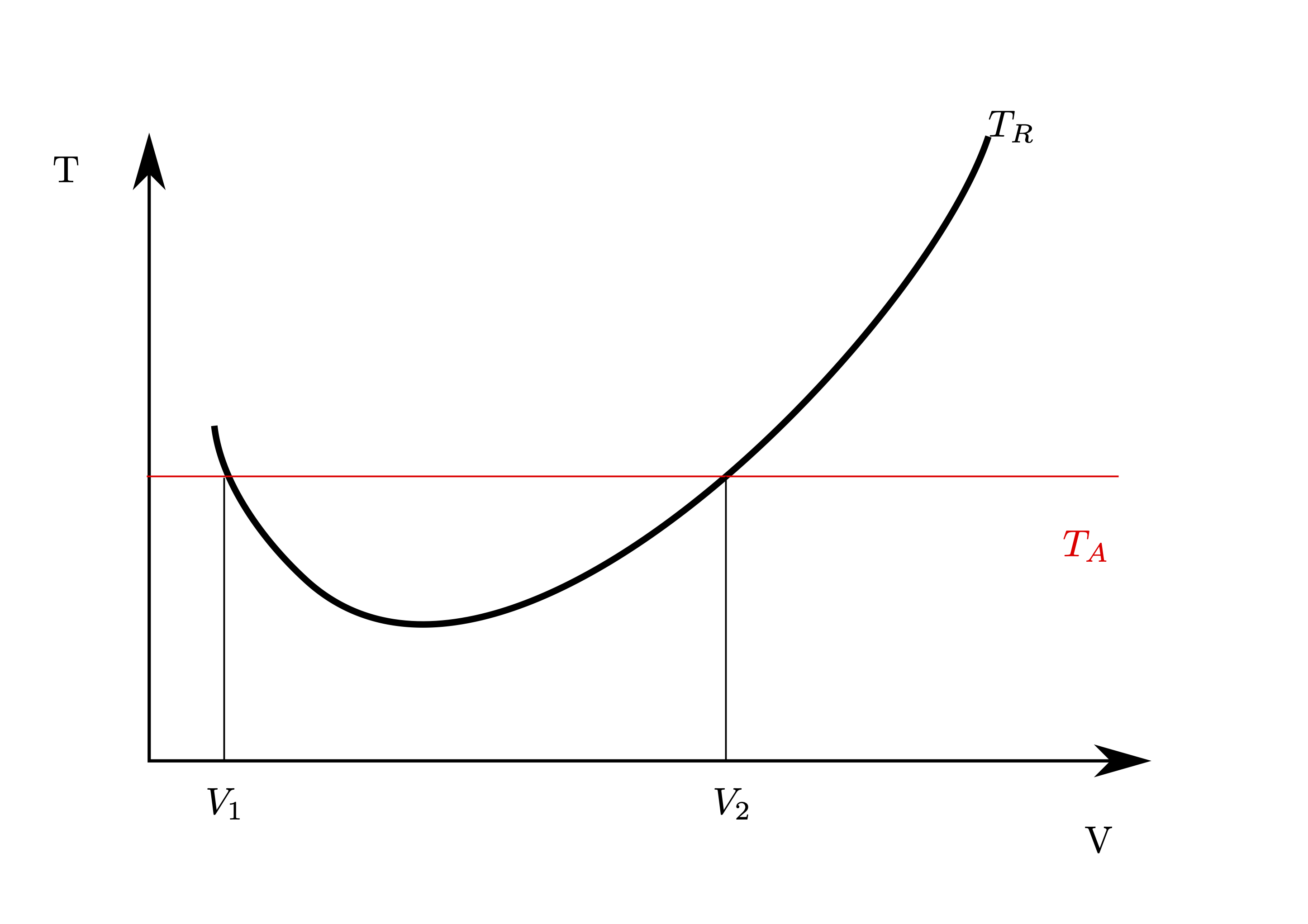
Fig. 19 Thrust Available and Thrust Required

Denoting the thrust produced by the powerplant as \(T_A\), meaning thrust available and the total drag as \(T_R\), meaning thrust required, the intersection between the \(T_A\) and \(T_R\) curves gives the possible flight speeds.

\(T_A\) is simply a number, whilst the \(T_R\) curve is a polynomial so the intersection can be determined from:

\[T_R=A\cdot V^2 + B\cdot V^{-2}\]

Which is equal to the thrust available:

\[T_R=A\cdot V^2 + B\cdot V^{-2}=T_A\]

\[A\cdot V^4 + B - T_A\cdot V^2=0\]

hence a quadratic in \(V^2\) or

\[a\cdot (V^2)^2 + b\cdot (V^2) + c=0\]

with \(a=A\), \(b=-T_A\) and \(c=B\)

\[V=\sqrt{\frac{T_A\pm\sqrt{T_A^2-4\cdot A\cdot B}}{2\cdot A}}\]

which yields the two velocities from the graph, \(V_1\) and \(V_2\).

Example

For an aircraft with a drag equation described by:

\[C_D = 0.016 + 0.045\cdot C_L^2\]

with a wing area of 50m\(^2\), a weight of 160kN, a \(C_{L,max}=1.5\), flying at sea-level determine the maximum and minimum flight speeds for a constant thrust of 10kN

Solution procedure - attempt the question before looking at the answer.

The drag equation gives you the constants \(C_{D0}=0.016\) and \(K=0.045\), and the remaining constants are provided in the question.

This enables you to determine the profile drag factor A=0.49000001 and the induced drag factor B=37616325.974.

With \(T_A=10,000N\), you now have everything to solve the quadratic equation to yield \(v_1=70.53m/s\) and \(v_2=124.43m/s\).

Look at the plot below, and see if you could reproduce is without looking at the source code.

import plotly.io as pio
import plotly.express as px
import plotly.offline as py
import plotly.graph_objects as go
from ambiance import Atmosphere
import numpy as np
import cmath

# Define constants
CD0=0.016 # Zero incidence drag
K=0.045 # Induced drag factor
S=50 # Wing area, m^2
W=160e3 # Aircarft weight, Newtons
Clmax = 1.5

alt=0; # Altitude

mosphere = Atmosphere(alt*1000)
rho = mosphere.density

# Determine stall speed
Vstall = np.sqrt(W / (0.5 * rho * S * Clmax))


# Determine A and B
A = CD0 * 0.5 * rho * S
B = K * W ** 2 / 0.5 / rho / S



# Flight speed vector
Vs = np.linspace(Vstall[0], 200, 1000)


# Define drags
Dind = B * Vs**-2
Dprof = A * Vs**2
D = Dind + Dprof

# Get minimum drag
Vmd = (B/A)**.25
md = A * Vmd**2 + B * Vmd**-2


fig = go.Figure()
# Thrust available
TA = 10e3
fig.add_trace(go.Scatter(x=[min(Vs), max(Vs)], y=[TA, TA], name="$T_A$", mode="lines"))

# Get the intersection
a = A
b = -TA
c = B
flight_limit_speeds = np.sort(np.sqrt(np.roots([a, b, c])))



fig.add_trace(go.Scatter(x=Vs, y=D, name="$T_R$"))
fig.add_trace(go.Scatter(x=Vmd, y=md, mode="markers+text", text="$V_{md}$", textposition="top center", name="Annotation"))

fig.add_trace(go.Scatter(x=flight_limit_speeds, y=[TA, TA], mode="markers+text", text=[f"V1={flight_limit_speeds[0]:1.2f}", f"V2={flight_limit_speeds[1]:1.2f}"], textposition="bottom center", name="Annotation"))



fig.update_layout(
    title=f"Graphical Solution",
    xaxis_title="TAS / (m/s)",
    yaxis_title="Drag / N",
    legend_title="Drag Breakdown",
)

for trace in fig['data']: 
    if(trace['name'] == "Annotation"): trace['showlegend'] = False

fig.update_xaxes(range=[0, 200])
fig.update_yaxes(range=[0, 20e3])

/Users/harrysmith/opt/anaconda3/lib/python3.8/site-packages/numpy/core/_asarray.py:136: VisibleDeprecationWarning:

Creating an ndarray from ragged nested sequences (which is a list-or-tuple of lists-or-tuples-or ndarrays with different lengths or shapes) is deprecated. If you meant to do this, you must specify 'dtype=object' when creating the ndarray

Speed stability in cruise

In the figure above, for a fixed throttle setting of 10kN, steady flight is possible at \(V_1\) or \(V_2\). At speeds \(V_1\) or \(V_2\) only \(T_A=T_R\) and there is no excess thrust.

At speeds \(V_1 < v < V_2\), there is positive excess thrust and at speeds \(v<V_1\) or \(v>V_1\) there is negative excess thrust (sometimes called excess drag). With positive excess thrust, the aircraft accelerates. With negative excess thrust the aircraft decellerates.

Flight at v1

Consider flight at \(V_1\) - any velocity perturbation (e.g., due to a gust) will move the aircraft into a condition of excess thrust.

For the case with no pilot input, if the aircraft speeds up, there will be positive excess thrust leading to acceleration all the way to \(V_2\). If the aircraft slows down, there will be negative excess thrust leading to decelleration all the way to \(V_{stall}\).

This is speed instability, and leads to increased pilot workload (requires continual throttle adjustments)

Flight at v2

Consider flight at \(V_2\) - any velocity perturbation (e.g., due to a gust) will move the aircraft into a condition of excess thrust.

For the case with no pilot input, if the aircraft speeds up, there will be negative excess thrust leading to decelleration back to \(V_2\). If the aircraft slows down, there will be postitive excess thrust leading to acceleration back to \(V_{2}\).

This is a stable system, with reduced pilot workload (no required throttle adjustments)

Stability boundary

Consider that the pilot may adjust the throttle to increase or decrease the thrust. Accordingly, if in the example given above the \(T_A\) line represents the maximum thrust, then the throttle could be adjusted to allow cruise to be possible at all speeds \(V_1\le v\le V_2\).

Using the reasoning above, though, it can be seen that cruise at any velocity \(V\leq V_{md}\) will be subject to a speed instability.

Caution - the above is a simplification.

The description of what happens with excess thrust as described above is a simplification (you’ll read this phrase a lot in Flight Mechanics).

In reality, whenever there is positive excess thrust, the resulting acceleration will result in a speed increase which, for a given attitude will result in an increase in lift and hence climb.

If the pilot wishes to maintain constant speed, they may intuitively adjust attitude via the stick/yoke which will take the aircraft out of equilibrium.

Aircraft Propulsion - thrust or power available

In the question above, it was assumed that the thrust was constant with forward speed. This is only the case for a pure turbojet or a high bypass-ratio turbofan. Before we can go further with the methodology, a broad comparison between aircraft powerplant types needs to be made.

With infinite thrust/power available, our aircraft could fly anywhere on the D vs. TAS curve, but this is not the case in reality. Thrust and power are provided by the aircraft powerplant, so some understanding of what it means to produce thrust is required.

Newton’s second law states that “force is equal to the rate of change of momentum”. The momentum change in question is that of the fluid before and the effect of the propulsor.

A revision of aircraft propulsion.

Recall that the fluid accelerates before and after the propulsor, and reaches the ultimate velocity at some downstream distance.

All generalised jets, meaning any propulsor that works by accelerating a fluid provide a \textsl{streamwise pressure discontinuity} which creates a continuous streamwise velocity variation. You may resolve the force as \(F=\Delta P\cdot A\) or \(F=\dot{m}\Delta V\), and these are equal to each other - they are not summative.

Defining a jet efflux velocity, \(v_j\), as the velocity of the air when it is fully accelerated by the propulsor. Newton’s second law is then:

\[\begin{split}\begin{aligned} T &= \frac{\text{d}}{\text{d}t}\left({m}\cdot\Delta v\right)\\ \text{in steady flight, }\Delta v=0\\ &= \dot{m}\cdot\Delta v \\ &= \dot{m}\Delta v\\ &= \dot{m}\left(v_j - V\right)\end{aligned}\end{split}\]

Considering work done; the work that the propulsor performs on the airframe is useful work, whilst any work done in providing the streamtube with velocity is waste work.

Work is force \(\times\) displacement in the direction of the force, and power is the rate of doing work, so:
Useful power

\[\begin{split}\begin{aligned} P &= T\cdot V\\ &= \dot{m}\cdot\left(v_j - V\right)\cdot V \end{aligned}\end{split}\]

Waste power is the rate of change of kinetic energy of the air:

\[\begin{aligned} P_{waste}=\frac{1}{2}\dot{m}\left(v_j-V\right)^2 \end{aligned}\]

Which allows the definition of propulsive efficiency as a measure of the propulsive power to the total power required.

\[\begin{split}\begin{aligned} \eta&=\frac{\text{Useful (Propulsive) Power}}{\text{Total Power Output}}\\ &= \frac{T\cdot V}{T\cdot V + \frac{1}{2}\dot{m}\left(v_j-V\right)^2 }\\ &= \frac{\dot{m}\cdot\left(v_j - V\right)\cdot V}{\dot{m}\cdot\left(v_j - V\right)\cdot V + \frac{1}{2}\dot{m}\left(v_j-V\right)^2 }\end{aligned}\end{split}\]

Noting that propulsive power is a function of the aerodynamics of the propulsor and does not include any effects such as losses in the powerplant itself.

Propellers and High Bypass-Ratio Turbofans have a high \(\dot{m}\) due to a large disc area, but a small \(v_j\). This means:

• Lower fuel consumption due to small KE increase

• Rapid loss of thrust with forward speed due to small \(v_j-V\)

These engines may be defined as power engines as their fuel consumption is generally linear with the power they produce. They have an associated specific fuel consumption (SFC) which has units of kg/s/W or lb/h/hP or equivalents.

Turbojets and Low Bypass-Ratio Turbofans have a small \(\dot{m}\) due to a small disc area, but a large \(v_j\). This means:

• High fuel consumption due to large KE increase

• Little loss of thrust with forward speed due to small \(v_j>>V\)

These engines are defined as thrust engines as their fuel consumption is generally linear with the thrust they produce. They have an associated thrust specific fuel consumption (TSFC) which has units of kg/s/N or lb/h/lbf or equivalents.

Thrust and Power Model

Since all aircraft propulsors accelerate a mass of air, it follows that their output is a function of air density/altitude - but also of many, many other factors.

Validity of this model

In reality, the relationships for thrust and power for different types of engines are functions of forward speed, Mach number, density, temperature, and engine-specific factors relating to efficiency.

For a detailed discussion of these effects, see Chapter 3 in “Aircraft Performance and Design” [And99]. The summary on page 186 results in the altitude model used in

There are a myriad of different thrust and power models used for aircraft performance, but for this course, the simplest one will be used.

For thrust engines, the altitude variation is described by:

\[\begin{split}\begin{aligned} \frac{T}{T_{SL}} &= k\cdot\sigma^n\label{eq:thrustmodel}\\ \text{where}\\ k &: \text{Throttle setting = 0 to 1}\\ T_{SL} &: \text{Thrust produced at ISA SL}\\ \sigma &: \text{Density ratio} - \frac{\rho}{\rho_{SL}}\\ n &: \text{1 if not indicated otherwise} \end{aligned}\end{split}\]

For power engines, the altitude variation is described by:

\[\begin{split}\begin{aligned} \frac{P}{P_{SL}} &= k\cdot\sigma^n\\ \text{where}\\ k &: \text{Throttle setting = 0 to 1}\\ P_{SL} &: \text{Power produced at ISA SL}\\ \sigma &: \text{Density ratio} - \frac{\rho}{\rho_{SL}}\\ n &: \text{1 if not indicated otherwise} \end{aligned}\end{split}\]

Some sources list \(n\) as an altitude dependent parameter that accounts for the change of lapse rate at the tropopause, whilst other list it as an engine-specific parameter. In this course, it will be used as a parameter that encompasses both - you will be able to assume \(n=1.0\) unless otherwise directed.

v1 and v2 with altitude

With the thrust or power model now giving the variation of available thrust with altitude (with the change in density), the range of possible speeds can be determined for different altitudes.

It can be appreciated that it is easier to perform this exercise in EAS rather than TAS, as there is a single \(T_R\) curve in EAS.

import plotly.io as pio
import plotly.express as px
import plotly.offline as py
import plotly.graph_objects as go
from ambiance import Atmosphere
import numpy as np
import cmath
from myst_nb import glue


# Define constants
CD0=0.016 # Zero incidence drag
K=0.045 # Induced drag factor
S=50 # Wing area, m^2
W=160e3 # Aircarft weight, Newtons
Clmax = 1.5

rho_sl = 1.225

TSL = 25e3

fig = go.Figure()


# Determine A and B - EAS
AE = CD0 * 0.5 * rho_sl * S
BE = K * W ** 2 / 0.5 / rho_sl / S

# Find mimimum drag as this sets the ceiling
Vemd = (BE/AE)**.25
Dmin = AE * Vemd**2 + BE * Vemd**-2
sig_dmin = Dmin/TSL
rho_dmin = sig_dmin * rho_sl

# Need to find the altitude for this - this isn't an efficient way to calculate it. But it'll work
ceiling_found = False
alt = 0
iteration = 0
dH = 1
while not ceiling_found:
    mosphere = Atmosphere(alt*1000)
    rho = mosphere.density
    drho = rho - rho_dmin
    dH = drho
    
    alt = alt + drho
    
    if abs(drho) < 1e-5:
        ceiling_found = True
    
ceiling = alt
altvec = np.arange(0, ceiling, 2)
altvec = np.concatenate((altvec, ceiling))

# Get minimum drag
Vemd = (BE/AE)**.25
md = AE * Vemd**2 + BE * Vemd**-2

# Turn this into TAS
Vmd = Vemd * sig_dmin**-.5

# Save these values for later
glue("Vemd", Vemd, display=False);
glue("Vmd", Vmd, display=False);




# Flight speed vector
# Determine stall speed
Vstall = np.sqrt(W / (0.5 * rho_sl * S * Clmax))
Vs = np.linspace(Vstall, 300, 1000)

# Define drags
Dind = BE * Vs**-2
Dprof = AE * Vs**2
D = Dind + Dprof

fig.add_trace(go.Scatter(x=Vs, y=D, name="$T_R$"))   



for alt in altvec:

    mosphere = Atmosphere(alt*1000)
    rho = mosphere.density

    # Thrust available at this altitude
    sigma = rho/rho_sl
    TA = TSL * sigma[0]

    # Plot available thrust
    fig.add_trace(go.Scatter(x=[0, 250], y=[TA, TA], name="Annotation", mode="lines"))
    fig.add_trace(go.Scatter(x=[250], y=[TA], mode="text", text=f"h={alt}km", textposition="middle right", name="Annotation"))
    
    # Get the intersection
    a = AE
    b = -TA
    c = BE
    flight_limit_speeds = np.sort(np.sqrt(np.roots([a, b, c])))
    
    # Is this in the envelope (this code is redundant now, but might be handy for later)
    in_envelope = not (isinstance(flight_limit_speeds[0], complex))
    
    # Add v1 and v2 annotations        
    if in_envelope and not (alt == ceiling):
        fig.add_trace(go.Scatter(x=flight_limit_speeds, y=[TA, TA], mode="markers+text", text=[f"v1={flight_limit_speeds[0]:1.2f}", f"v2={flight_limit_speeds[1]:1.2f}"], textposition="bottom center", name="Annotation"))
    elif in_envelope:
        fig.add_trace(go.Scatter(x=[flight_limit_speeds[0]], y=[TA], mode="markers+text", text=[f"v1=v2={flight_limit_speeds[0]:1.2f}"], textposition="bottom center", name="Annotation"))


# Add the stall speed
fig.add_trace(go.Scatter(x=[Vstall, Vstall], y=[0, 30e3], mode="lines", name="Annotation"))        
fig.add_trace(go.Scatter(x=[Vstall], y=[27e3], mode="text", text="Stall Speed", textposition="middle right", name="Annotation"))

fig.update_layout(
    title=f"$T_R \\text{{ and }} T_A \\text{{ for different altitudes}}$",
    xaxis_title="EAS / (m/s)",
    yaxis_title="Drag / N",
    legend_title="Drag Breakdown",
)

for trace in fig['data']: 
    if(trace['name'] == "Annotation"): trace['showlegend'] = False

fig.update_xaxes(range=[0, 260])
fig.update_yaxes(range=[0, 30e3])

fig.show()

Look at the graph above, observe the following:

• There is a single \(T_R\) curve since the graph has been plotted in EAS

• At sea-level the \(T_A\) curve is highest as the air density is lowest, hence there is the greatest available thrust

• As altitude increases, the available thrust decreases, and hence the minimum flight speed \(v_1\) increases whilst the maximum flight speed \(v_2\) increases

• For many altitudes, the minimum flight speed is lower than the stall speed hence the value has no physical significance - since flight would not be possible at these speeds

• Altitudes have been plotted in 2km intervals, which is an arbitrary interval.

• As \(v_1\) and \(v_2\) get closer together, they finally meet at the minimum drag speed - the physical significance here is that at this altitude the engine can only produce sufficient thrust (i.e., at maximum throttle) to enable cruise at a single speed (that which requires the minimum thrust, \(V_{md}\)) - 93.604m/s EAS or 159.719m/s TAS

Plotting flight speeds

From the above, it is possible to plot the maximum and minimum flight speeds with altitude

# Make a vector for the altitude in 100m intervals
alt_vector = np.arange(0, ceiling, 0.1)
alt_vector = np.concatenate((alt_vector, ceiling))

# AE and BE are already available from before - we'll introduce two new arrays to store V1 and V2
#EAS
VE1 = np.zeros(alt_vector.shape)
VE2 = np.zeros(alt_vector.shape)

#TAS
V1 = np.zeros(alt_vector.shape)
V2 = np.zeros(alt_vector.shape)

# iterate over the altitudes
for i, altitude in enumerate(alt_vector):
    mosphere = Atmosphere(altitude*1000)
    rho = mosphere.density

    # Thrust available at this altitude
    sigma = rho/rho_sl
    TA = TSL * sigma[0]
    
    # Get the intersection
    a = AE
    b = -TA
    c = BE
    flight_limit_speeds = np.sort(np.sqrt(np.roots([a, b, c])))
    
    # Store these in the array
    VE1[i] = flight_limit_speeds[0]
    VE2[i] = flight_limit_speeds[1]
    
    # And for EAS
    V1[i] = VE1[i] * sigma ** -.5
    V2[i] = VE2[i] * sigma ** -.5
    
    
# Sort these into an array for plotting
VEs = np.concatenate((VE1, np.flip(VE2)))
Vs = np.concatenate((V1, np.flip(V2)))
alt_vector = np.concatenate((alt_vector, np.flip(alt_vector)))

# 



fig = go.Figure()

fig.add_trace(go.Scatter(x=VEs, y=alt_vector, mode="lines", name="EAS"))
fig.add_trace(go.Scatter(x=Vs, y=alt_vector, mode="lines", name="TAS"))

fig.update_layout(
    title=f"Possible airspeeds for different altitudes in EAS and TAS",
    xaxis_title="Airspeed / (m/s)",
    yaxis_title="Altitude / km",
)

    

Now - the plot above show the possible flight speeds from the solution of the quadratic, but it was shown in the previous plot that for lower altitudes, \(v_1\) was below the stall speed.

If this is taken into consideration, then the plot is modified to:

The source code for the plot above is not included on the website - though you could download it if you look at the source .ipynb file.

You are advised to try and reproduce the plot above based on the source code from the previous plot. This will be a good test of your ability to understand the equations and the logic flow of these codes.

Aircraft Absolute Ceiling

This introduces the concept of aircraft absolute ceiling, which is defined as the altitude at which the only possible flightspeed is \(V_{md}\).

A consideration of this concept should ring alarm bells in your aircraft performance engineer’s brain.

What alarm bells?

Think back to the concept of speed stability - where the idea of velocity perturbations were introduced.

If an aircraft is flying at the absolute ceiling, then any velocity perturbation will push the aircraft to a speed where there is negative excess thrust and thus the aircraft will begin to sink.

As a consequence, sustained cruise at the absolute ceiling is not feasible.

For the above reasons, the aircraft absolute ceiling is rarely used or listed by a manufacturer. In reality, the aircraft service ceiling is defined, where a small rate of climb is still possible - the rate is usually dictated by the manufacturer.

To explore this concept, a model for climbing/sinking/gliding flight will be required. This ends the section of Steady Level Flight.

Defining Aircraft ‘Speed’ Climbing and Gliding Caveat