Climbing and Gliding Caveat#
Since this course comprises both aircraft performance and flight mechanics, the nomenclature can be a little confusing when trying to keep things consistent across the disciplines.
Aircraft performance uses simplified models of aircraft mechanics to determine basic relationships for flight. Using these to predict climbing and gliding flight is possible, and will be completed in the following, but some explanation of the nomenclature will be described first.
Flight Mechanics Angles#
To describe the aircraft attitude a set of angles are used called Euler angles - these will be fully described in Module 3. The aircraft pitch is defined as the angle between the horizontal and the earth axis, and is given the symbol \(\theta\).
To describe the aircraft flight path a set of angles describing the orientation of the aircraft velocity vector with respect to the earth are used. These are the flight path angle \(\gamma\), and the track angle, \(\tau\).
To describe the aerodynamic incidence, the aerodynamic angles \(\alpha\) and \(\beta\) are used. \(\alpha\) is angle of attack, and \(\beta\) is sideslip.
The angles above will be fully explored and utilised in the later modules, but an appreciation of the longitudinal angles is required here:
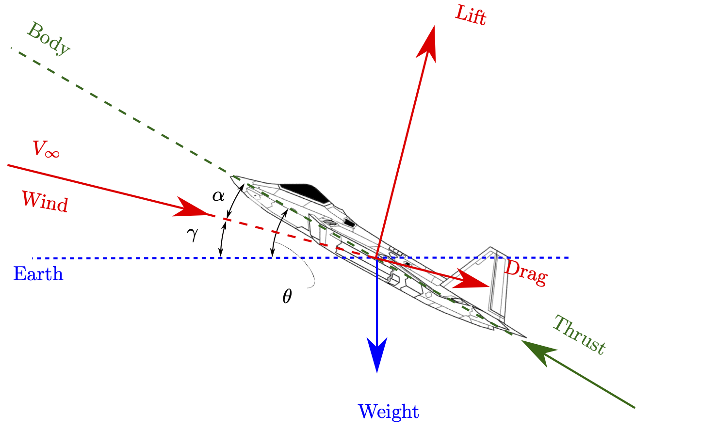
Fig. 20 Relationship between longitudinal angles#
Aircraft Performance#
In aircraft performance, the climb or glide angle is denoted by \(\theta\) in numerous texts - for example - and this angle represents the angle between the aircraft flight direction and the horizontal plane.
Looking at Fig. 20, you will see that this should really be denoted by \(\gamma\). In the following, the glide or climb angle will be denoted by \(\gamma\), but you should be aware that in most texts you will see it denoted by \(\theta\).
In reality, \(\gamma=\theta\) if and only if (iff) \(\alpha=0\).
The distinction is made because this course later requires us to use \(\theta\), and I don’t want you getting confused about what the angles mean.
Since the flight path angle, \(\gamma\), is defined as positive in a glide and negative in a climb (positive \(\gamma\) gives positive \(W_e\) which is velocity towards the earth), it leads to requiring a negative angle continually in the climb expressions. uses a good approach and introduces
to avoid the negative expression. For the following, \(\bar{\gamma}\) will be used.
Gliding Flight (Unpowered Descent)#
The parameters determine above, the lift and hence speeds for minimum thrust and minimum power are important for determination of an aircraft’s glide characteristics.
Why gliding?
If you’ve never experienced flight in a glider, I’d thoroughly recommend it (I’m a recent convert to gliding from powered flight).
It will make you a more rounded aeronautical engineer, and enable you to fully understand the significance of the parameters we’re talking about here.
I’m trying to get a flying club set up for our school, so hopefully it’ll happen soon…
With no thrust, the aircraft has \(T=0\) but \(D>0\), so there is no longer force equilibrium. The aircraft will descend at the glide angle \(\bar{\gamma}\). In a steady glide, the horizontal component of weight is equal to the drag.
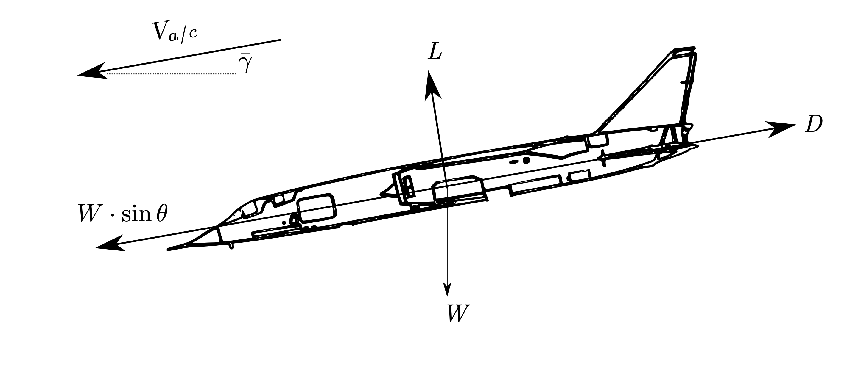
Fig. 21 Forces on aircraft in a glide#
What’s actually happening in a glide?
In the preceding section, the aircraft was in equilibrium - the lift was equal to the weight, and the thrust was equal to the drag.
Drag is the aerodynamic force opposing motion, and has an associated power - which is the rate that the aircraft does work on the flow in the direction of motion. During cruise, the thrust power (\(T\cdot V\)) is equal to the power associated with drag.
With no input power (\(T=0\)), in order to maintain a constant forward speed, some power has to be input to the aircraft to maintain horizontal equilibrium. As stated, part of the weight vector (\(W\cdot\sin\bar{\gamma}\)) opposes the drag.
The associated power the rate of change of gravitational potential energy. In a glide, potential energy is being exchanged for kinetic energy to maintain forward speed.
Glide Angle#
In Fig. 21, the forces are parallel and perpendicular to the flight path as before, but you should note that this is no longer parallel with the ground. In the horizontal direction, equilibrium gives \(W\cdot\sin\bar{\gamma}=D\) and in the vertical direction, equilibrium gives \(L=W\cdot\cos\bar{\gamma}\). Hence the glide angle can be determined from simple trigonometry:
So it can be seen that the best/shallowest glide (the smallest \(\bar{\gamma}\)) occurs at the minimum drag to lift ratio - i.e., at \(C_{L,md}\).
The glide angle dictates the glide distance, which is very important to be aware of in the cockpit in a glider as this dictates the furthest distance that can be covered along the ground.
The aircraft speed equation can be used with \(L=W\cdot\cos\bar{\gamma}\) in place of \(L=W\) - which shows that the speed that the shallowest glide occurs is not \(V=V_{md}=\left[\frac{B}{A}\right]^\frac{1}{4}\) as \(V_{md}\) as calculated previously is only valid for cruise.
Small angle assumption?#
The speed for minimum slide is therefore slower than the minimum drag speed in cruise. Compare the ratio of the two speeds for a range of glide angles:
Show code cell source
import numpy as np
import plotly.graph_objects as go

# Make a vector of reasonable glide ratios - say 30 - 80
glide_ratios = np.linspace(2, 80, 1000)
glide_angles = np.arctan(1/glide_ratios)

Vbestglide_on_Vmd = np.sqrt(np.cos(glide_angles))


fig = go.Figure()
fig.add_trace(go.Scatter(x=glide_ratios, y=glide_angles*180/np.pi))

fig.update_layout(
    title="Glide Angle vs. Glide Ratio",
    xaxis_title="Glide Ratio",
    yaxis_title="Glide Angle / deg",
)

fig.show()

fig = go.Figure()
fig.add_trace(go.Scatter(x=glide_ratios, y=Vbestglide_on_Vmd))

fig.update_layout(
    title="$\\text{Ratio of best glide speed and }V_{md}$",
    xaxis_title="Glide Ratio",
    yaxis_title="$\\frac{V_{bestglide}}{V_{md}}$",
)

fig.show()
It can be seen that for glide angles up to around 11 degrees, the best glide speed is 99% of \(V_{md}\). So for most glide performance work, it is assumed that the shallowest glide occurs at \(V_{md}\).
Since most performance gliders have great glide ratios (\(\frac{C_L}{C_D}\)), the above small angle approximation is suitable for gliders and aircraft with reasonable glide ratios. It may not hold for some other aircraft, however, in which case the shallowest glide speed of \(V_{md}\sqrt{\cos\bar{\gamma}}\) must be used.
Sink rate#
Whilst the glide angle dictates the distance along the ground (hence giving the range), the best endurance is given by the slowest overall descent. Thus the sink rate needs to be minimised.
The sink rate, \(V_{sink}\), is the vertical component of flight speed - \(V_{sink}=V\cdot\sin\bar{\gamma}\). From the reasoning used previous regarding the exchange of potential energy for kinetic energy, you should be able to intuit that the minimum sink rate occurs at the minimum power speed.
Intuition and mathematics
This is a great example of how you should approach these sorts of problems. We know from logical reasoning that the minimum sink rate must occur at the minimum power speed.
So we’ll go through the mathematics and we should find that \(V_{minsink}=\left[\frac{B}{3\,A}\right]^\frac{1}{4}\).
If we find anything else, either we have made a mistake or there is a flaw in our assumptions or reasoning.
The sink rate is the vertical component of flightspeed, \(V_{sink}=V\cdot\sin\bar{\gamma}\) - see Fig. 22
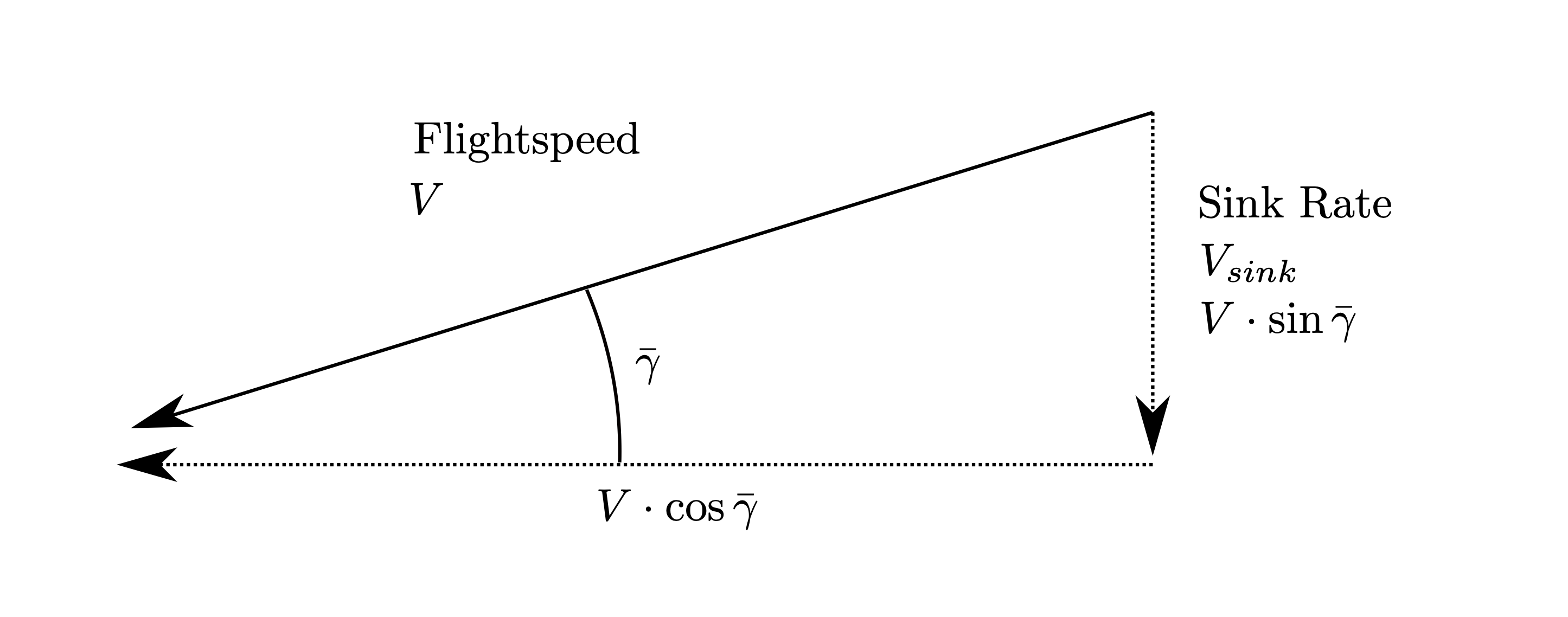
Fig. 22 Glide Velocities#
so
from equilibrium and making the small angle assumption for \(\bar{\gamma}\)
using the aircraft speed equation and using the small angle assumption to substitute \(L\simeq W\)
since the other terms are just constants, or outside of our control, then the minimum sink rate is found at the minimum of \(\frac{C_D}{C_L^{3/2}}\) which can be found from some elementary calculus by substituting \(C_D=C_{D0}+K\cdot C_L^2\) and differentiating by \(C_L\):
Substitution of this into the aircraft speed equation, Eq. (5), yields the speed for minimum sink
which is equal to \(V_{minsink}=\left[\frac{B}{3\,A}\right]^\frac{1}{4}\), or the minimum power condition, which is what was expected from intuition.
Small angle assumption?
See if you can determine the relationship between \(\frac{V_{minsink}}{V_{mp}}\) if the small angle assumption cannot be used.
Glider Polar#
For the pilot, as has been mentioned previously, the actual lift coefficient or angle of attack for a given condition is not usually of relevance. A glider pilot will be keenly aware of their best sink rates, and will desire to know the airspeed(s) at which these occur.
Glider manufacturers tend to provide a chart of sink rate vs. airspeed, which is proportional to the \(\frac{D}{L}\) ratio against the inverse of the lift coefficient (with some additional exponents thrown in for good measure).
Show code cell source
# Aircraft Input data - representative glider data taken from https://booksite.elsevier.com/9780123973085/content/APP-C4-DESIGN_OF_SAILPLANES.pdf page 23
# and from Stemme S10 info at https://en.wikipedia.org/wiki/Stemme_S10
#
# Note that I have reduced the stall speed slightly to show the shape of the drag polar in more detail
CD0 = 0.008
e = 0.95
AR = 28
W = 850 * 9.80665 # Gross weight
Vstall = 35 # knots
Vne = 146 # knots
S = 18.7
rho_sl = 1.2255

# Get the induced drag factor from Oswold efficiency
K = 1/np.pi/e/AR


# Make a vector of speeds
Vknots = np.linspace(Vstall, Vne, 1000) # In knots
Vms = Vknots * 0.5144444 # In m/s

# Get the CL values for these speeds
CLs = 2*W/rho_sl/S/Vms**2

# Get the corresponding drags
CDs = CD0 + K * CLs**2


# Determine the sink rates
w_e = np.sqrt(2 * W / rho_sl / S) * CDs / CLs**(3/2) / 0.5144444

#### Get points for min glide angle
# Get ClMD and associated sink rate for plotting
A = .5 * CD0 * rho_sl * S
B = K * W**2 / rho_sl / 0.5 / S

# Minimum drag speed
Vmd_ms = (B/A)**(1/4)
Vmd_knots = (B/A)**(1/4) / 0.5144444

# Associated Cl and Cd
Clmd = np.sqrt(CD0/K)
Cdmd = CD0 + K * Clmd**2

# Sink rate at minimum drag speed
w_emd = np.sqrt(2 * W / rho_sl / S) * Cdmd / Clmd**(3/2) / 0.5144444

#### Do the same for the minimum sink rate
# Minimum power speed
Vmp_ms = (B/3/A)**(1/4)
Vmp_knots = (B/3/A)**(1/4) / 0.5144444

# Associated Cl and Cd
Clmp = np.sqrt(3*CD0/K)
Cdmp = CD0 + K * Clmp**2

# Sink rate at minimum power speed
w_emp = np.sqrt(2 * W / rho_sl / S) * Cdmp / Clmp**(3/2) / 0.5144444

# Make a plot
fig = go.Figure()
fig.add_trace(go.Scatter(x=Vknots, y=w_e, name=f"Gross weight = {W}N"))


# Annotate it
fig.add_trace(go.Scatter(x=[Vmd_knots], y=[w_emd], mode="markers+text", text=f"Vmd={Vmd_knots:1.2f}kn$", textposition="middle right", name="Annotation"))
fig.add_trace(go.Scatter(x=[Vmp_knots], y=[w_emp], mode="markers+text", text=f"Vmp={Vmp_knots:1.2f}kn$", textposition="middle right", name="Annotation"))

# Draw a line to the minimum drag speed
fig.add_trace(go.Scatter(x=[0, Vmd_knots*2], y=[0, w_emd*2], mode='lines', name="Annotation"))


fig.update_layout(
    title="Glider Polar",
    xaxis_title="Airspeed kn EAS",
    yaxis_title="Sink rate kn EAS"
)


fig.update_yaxes(range=[2.5, 0])
fig.update_xaxes(range=[0, 150])

for trace in fig['data']:
    if(trace['name'] == "Annotation"): trace['showlegend'] = False

fig.show()
You can see that an increase in the aircraft weight moves the curve along so its tangent remains the same.
Note: The weights for the plot are likely unfeasible for this aircraft but they make for a nice plot
Powered Descent#
The procedure for powered descent and determination of descent slope and sink rate is the same but with \(D=T + W\sin\gamma\)