Introduction to this website

If you’ve stumbled across this website, then you’re in for a treat - provided you actually want to learn about Flight Mechanics.

This website was the course notes for my old class, Aircraft Flight Mechanics when I taught at Illinois Tech. I put everything online because I believe information like this should be available freely, and I think it’s a good way to share content by contrast to a book. Despite being OK at being a professor I no longer teach for a living, and I am now happily employed at Aurora Flight Sciences, a Boeing Company. But I still find my own notes useful, and I often direct junior engineers here to explain concepts…and to help me earn the occasional cent from ad revenue ;).

I will be updating this website slowly but surely as my own knowledge develops. This website will not contain any new code I’ve developed during the course of my employment, but as I find out useful things that are in the public domain, then I’ll put them up here.

Some folks have already been in touch and kindly highlighted errata in this website, too, and I will get on with making those changes as and when I can.

The old introduction

This obviously ain’t current any more

This website comprises the course notes for MMAE 410 Aircraft Flight Mechanics at the Illinois Institute of Technology - this text originally started as a PDF file written using LaTeX, with links to code and other tidbits. These notes started as my means of ensuring my own competence with the material and, accordingly, they get updated regularly and requiring students to download an updated PDF file every few weeks proved to not be the ideal solution.

So now these notes are being transferred into Jupyter notebooks which are bundled together into this document - any changes made to the notes should be reflected in the website within minutes, and this format allows handy things like interactive content, which simply isn’t possible (easily) within a PDF.

It does mean that my pipedream of getting them published as a textbook is over - but in the spirit of open access and education for all, I’d simply rather that they just got used for their intended purpose. Hence; use these notes to supplement your own learning, and to further your knowledge of the discipline.

Note: these are getting written and updated as the course is being taught, so they’re only as up-to-date as they need to be\

Due to COVID-19, my Fall 2020 class is entirely online - and I’ve chosen to pre-record all my lectures, which will be available on YouTube, and will get updated as I record/release them in batches.

For students in the class at IIT, there is content available via Slack and I will be hosting regular review sessions via Zoom.

In the interest of open access, I’ve decided to release my lectures for all in addition to this content.

The review sessions, Slack space, and assessment is available to enrolled students only.

Technical Computing - Why all the Python?

There is a lot of ‘pen and paper’ content in this work, and you need to go through the derivations yourself and understand the mathematics. The accompanying lectures cover the mathematical derivations and do work on the ‘whiteboard’ (which is actually an iPad).

With modern engineering, though, there’s a limit reached very quickly with what you can do by hand. Even simple hand calculations are often faster to complete using some form of tehcnical computing - especially if you have to repeat them. With this in mind, I try and instill in my students a will to use computing at every level. That is; I want you to be able to solve problems by hand, and also solve them using some form of technical computing.

You can choose whatever environment works for you; lots of engineers use Excel to do things that they shouldn’t (I’ve seen a propeller wake model written using Excel macros), and I have been guilty of using MATLAB to do things that I shouldn’t have (such as batch-renaming files, or automating the e-mail of grades to students).

The original PDF notes were written and contained examples using both MATLAB and occasional Python. Over the past few months, I’ve made the personal decision to switch all my code from MATLAB to Python. There are many reasons for this change, but the benefit for the reader is that you can view and run the source for any of the plots included in this online book without purchasing a MATLAB license.

I’ve discovered that Python is a wonderful and extensible programming language, which can be used to replicate pretty-much all of the functionality in MATLAB - often much more elegantly because of the nature of the language itself. MATLAB, on the other hand, is easy to get started with to perform calculations and you can construct some wonderful programs using MATLAB - but it’s not a very good programming language, which is a common opinion.

So - the choice is yours; you should complete the exercises using some form of technical computing. I don’t mind what you use, as long as you get the work done. I will offer accompanying examples that will help you understand all the problems, and these will be written in Python. The original MATLAB codes should still be available in the PDF notes.

As an aeronautical or mechanical engineering student, you should be good at coding - it will help you in your studies, and it will help you in your career. For example, if you want to practice problems for an examination - re-write an example using some programming language, and you can then simply change the input numbers and you’ll have a whole set of answers to check your work against.

Another Python vs. MATLAB bit of snark

Let’s do another quick pointer as to how Python has some cool features that MATLAB really struggles with. Let’s say you wish to switch the value of two variables. This is a simplified version of the core operation that you need to perform when you do an Euler Transform. In Python, you can update multiple variables at once based on the current values of those same variables.

What on earth does that mean?

a = 1
b = 2
c = 3
print(f"Before switching, a={a}, b={b}, c={c}")

a, b, c = c, a, b

print(f"After switching, a={a}, b={b}, c={c}")

Before switching, a=1, b=2, c=3
After switching, a=3, b=1, c=2

Try and do the same line in MATLAB - it will print the current values of all three values and do dick-all about changing their values. Superb. It basically sees this and says

sure, I'll print a, then b, I'll set c = c and then print it because you forgot a semicolon, then I'll print a, and b again. That'll be several thousands of dollars a year, please.

It might not seem that useful to be able to do this - but consider a basic Euler Transform. In Python you can now do something like

import numpy as np
ang = np.radians(45)
X = 1
Y = 2
X, Y = np.cos(X) - np.sin(Y), np.cos(Y) + np.sin(X)

whereas in MATLAB you’re forced to replace that single line either with some an array operation or do something like Xold=X and so on. Rant over.

Matplotlib or Plotly

You will see that I have chosen to use plotly to produce a lot of the figures in this online textbook. There were several reasons for this:

• Plotly allows the figures to be interactive in that you can zoom, pan, hide/show different traces

• Plotly allows the figures to be updated with live data, so this should allow further interactivity

• I fancied a challenge

There is a drawback to this in that I find plotly to produce plots that aren’t quite so suitable for presentation by contrast to matplotlib. This means that you should probably use matplotlib when submitting homework as a PDF.

This actually makes it a benefit for me as an instructor in that you should use the source code to see how the plots are made, but then write your own using matplotlib or MATLAB or whatever.

Interactive content

There is iteractive content that will help you to explore equations, and understand the relationship between different parameters.

The way this works is slightly convoluted, but very powerful - this whole book is hosted as a GitHub repository, as a mixture of .md and .ipynb files. This means that any Jupyter Notebooks can be run on the web thanks to the kind folks at DockerHub. The book is written using JupyterBook, which is a plugin called thebe, which enables the code sections to be run without having to actually go to DockerHub.

What this means is that you have a few different ways to access the interactive content:

• Download the whole .ipynb file and run natively in Juypter on your machine

• Run the notebook in Docker

• Run the code in-place using thebe

Both of the latter work well on the pages I have tested - but it can take time for the whole notebook to be initlialised. If you click on “run code” in the dropdown from the rocket icon at the top of the page, it needs to connect to Docker, which then connects to GitHub, and then send the content back to this site.

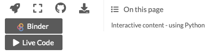
Fig. 1 Connecting to Binder/Thebe

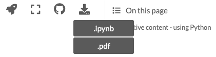
Fig. 2 Downloading the source or a PDF

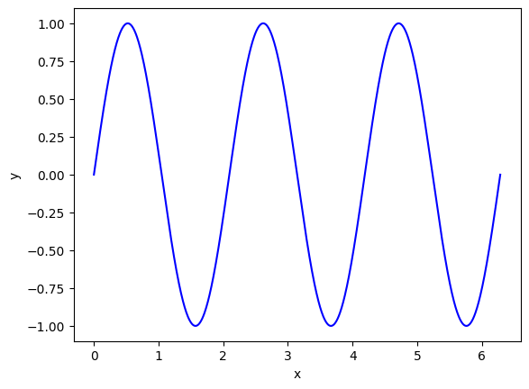
Give it a go, though - here’s a trivial example of a plot that you can edit. Try the different ways of accessing this content.

The plot below plots \(y=\sin(n\cdot x)\) in the interval 0 to \(2\pi\). You can change whatever you want in the code below and make it run.

import numpy as np
import matplotlib.pyplot as plt

n = 3

x = np.linspace(0, 2*np.pi, 1000)
y = np.sin(n * x)

plt.figure()
plt.plot(x, y, '-b')
plt.xlabel('x')
plt.ylabel('y')

Text(0, 0.5, 'y')

or we can use the much fancier but horrendously syntaxed Plotly. The syntax is like a second language to me now, but it’s not intuitive if you grew up with MATLAB.

import plotly.graph_objects as go

fig = go.Figure()
fig.add_trace(go.Scatter(
                        x = x,
                        y = y,
                        name="sin x"))
fig.update_layout(
    title="A slightly-fancier version of the plot from before",
    xaxis_title="x",
    yaxis_title="y",
)
fig.show()

_Note: this website is provided for free, and the ad revenue doesn’t get close to the annual hosting cost - let alone my effort involved. If you find these notes useful, and didn’t have to buy a textbook or similar because of it, then please consider buying me a coffee or…more likely…a beer